Launch Day Github Updates!

New to the Github for launch day:  a new processing workflow, and simulator v2.0!

The Processing workflow

The processor script's role in the backtesting process is to take a list of instances (which up until now have always been hold levels, but they could be any candle pattern you can think of) and find out what happened to them.  The previous version would start on its pending date and scan for an activation, and then it would check a few standard levels of retracement (fib 0.5, 0, -0.5, -1) on the way to reaching target (1.618), recording target/timestamp combinations.  All of this was hardcoded - the status flow, the retracement levels.  We needed something more robust.

The new processing workflow breaks the code up into a few components; the important parts are:

• The processing_timestamps_library.py file contains the main functions to find targets and timestamps.  It uses a "gear-shifting" approach to searching for targets, starting on the 1-second data (if you have it, best guess if you don't), gearing up to 1m, then 30m, then 1D.  When it finds its target on a higher timeframe, it then gears down to smaller timeframes until it arrives at the precise moment the level was reached.  It takes a start date and an optional end date for each search.
    It now has five modes:
  • • search a single direction (find an activation)
    • bidirectionally (target or SL?)
    • race a target in one direction versus a candle closing below a specified level in the other direction.
    • race a target in one direction versus a hard close below a specified level.
    • level sequence processing (more on this later)
• run_processing.py is the executable that launches a processing run, by specifying your configuration file with --config <relevant path to your config file>

Configuration files can now define any sort of processing you want to do.  For example, to process the standard levels from the previous version of the script, we could define our configuration as a series of tasks and actions, like this:

• Task 1: search for activation at fib 1.0 (single direction).  When it is found, perform the following actions:
  • • record active date
    • set status to active
• Task 2: search for completion at fib 1.618 versus retracement to fib 0.5, starting from activation date.
  • • If fib1.618 is first,
      • • record completed date
        • set status to completed
        • exit processing
    • if fib 0.5 is first,
      • • record date reached fib 0.5
        • Go to task 3
• Task 3: search for completion vs retracement to fib 0, starting at date reached fib 0.5.

etc, etc.  Task 4 for fib -0.5, task 5 for fib -1.0, and then...

• Task 6: final completion check - does it ever reach target from beyond fib -1.0? (single direction)

If instead of ending processing when the instance is completed you wanted to test extended TP strategies, you could re-route your tasks 2-6 to send you to a 7th task where you start from the completed date, and check fib 2.618 versus a retracement back to fib 1.0 or wherever.  You could set up multiple levels of retracement to test just like we did with the levels 0.5, 0, -0.5, -1.0 above.

So all of that to say, the processing workflow is very flexible:  any level, in any order, with any prerequisites you can imagine.  You can even invent your own arbitrary statuses for the processing and have them assigned as appropriate.

Simulator 2.0

In the new version of the simulator, we no longer use the entirety of config.py to define a single strategy; instead we can define multiple entry and exit strategies, or counter strategies, in a single configuration file and run them all in one simulation.

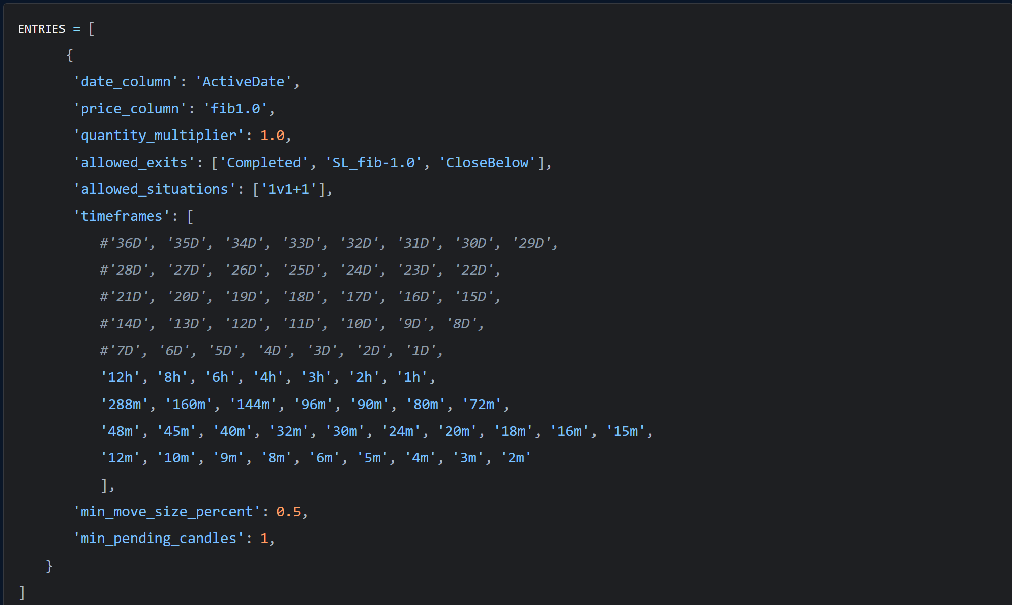
So while some variables remain global, like instance paths, max leverage, or start/end dates, other variables are now on a per-"entry strategy" basis.  Entries are defined with a target / timestamp, a list of named exits the entry can take, and other filters.  For example:

ENTRIES = [
       {
        'date_column': 'ActiveDate',
        'price_column': 'fib1.0',
        'quantity_multiplier': 1.0,
        'allowed_exits': ['Completed', 'SL_fib-1.0', 'CloseBelow'],
        'allowed_situations': ['1v1+1'],
        'timeframes': [
            #'36D', '35D', '34D', '33D', '32D', '31D', '30D', '29D', 
            #'28D', '27D', '26D', '25D', '24D', '23D', '22D', 
            #'21D', '20D', '19D', '18D', '17D', '16D', '15D', 
            #'14D', '13D', '12D', '11D', '10D', '9D', '8D',
            #'7D', '6D', '5D', '4D', '3D', '2D', '1D',
            '12h', '8h', '6h', '4h', '3h', '2h', '1h',
            '288m', '160m', '144m', '96m', '90m', '80m', '72m',
            '48m', '45m', '40m', '32m', '30m', '24m', '20m', '18m', '16m', '15m',
            '12m', '10m', '9m', '8m', '6m', '5m', '4m', '3m', '2m'
            ],
        'min_move_size_percent': 0.5,
        'min_pending_candles': 1,
    }
]

We can also now define "counter-trade" entries, too.  With this one we're again just specifying a target & timestamp pair and other filters, and simply reversing the direction of the instance (longing a short instance, shorting a long instance).

CT_ENTRIES = [
    {
        'date_column': 'CloseBelowDate',
        'price_column': 'CloseBelowPrice',
        'quantity_multiplier': 0.5,
        'allowed_exits': ['CTBoundaryHit'],
        'conditions': [("CloseFibLevel", "<=", 0.5), ("CloseFibLevel", ">=", -1.5)],
        'allowed_situations': ['1v1+1'],
        'timeframes': [
            #'14D', '13D', '12D', '11D', '10D', '9D', '8D',
            '7D', '6D', '5D', '4D', '3D', '2D', '1D',
            '12h', '8h', '6h', '4h', '3h', '2h', '1h',
            '288m', '160m', '144m', '96m', '90m', '80m', '72m', 
            '48m', '45m', '40m', '32m', '30m', '24m', '20m', '18m', '16m', '15m',
            '12m', '10m', '9m', '8m', '6m', '5m', '4m', '3m', '2m'
        ],
        'min_move_size_percent': 0.5,
    },
]

And the exits are simply defined as a target / timestamp pair, and given a name that they can be referred to in the entry definitions:

EXITS = [
    ("CompletedDate", "fib1.618", "Completed"),
    ("DateReached-1.0", "fib-1.0", "SL_fib-1.0"),
    ("CloseBelowDate", "CloseBelowPrice", "CloseBelow"),
]

# Counter-Trade Exits - same format as EXITS, used only by CT positions
CT_EXITS = [
    ("BoundaryHitDate", "BoundaryHitPrice", "CTBoundaryHit"),
]

By adding the quantity multiplier option, you can now specify advanced TP strategies or layering into an entry in your simulation.  Here is an example of a multi-layered exit strategy:

Entry definition #1: enter on fib 1, exit on SL or completed; quantity multiplier 0.75  (ie take 75% at TP1)
Entry definition #2: enter on fib 1, exit on SL or when TP2 is reached or on a retrace to fib 1 after completed; quantity multiplier 0.15 (ie take 15% at TP2 and exit if it returns to fib 1 after TP1)
Entry definition #3: enter on fib 1, exit on SL or when TP3 is reached or on a retrace to TP1 after TP2; quantity multiplier 0.1 (take 10% at TP3 or if it returns to TP1 after TP2)

Because the original simulator didn't quite get that entries / exits are a target / timestamp pair, it is no longer recommended for use, as it makes bad assumptions on exit prices.

Samples Included

The github has been loaded with a few sample processing configurations:

• standard instance processing; the new version of the hardcoded original script, in both .json and .yaml format
• a version of standard processing that includes a check for a close below entry (more on this coming in the next post!)
• a version of standard processing that includes a basic extended TP strategy
• a sample of level sequence processing (which tests for bounces between levels, but won't be covered in this post)

Questions, comments, ideas?  Let's talk about it in the Discord server!  Come find us at https://discord.gg/fiblab